Important Measures of Transport Networks

Network analysis is an important aspect of transport geography because it involves the description of the disposition of nodes and their relationships and line or linkage of distribution. It gives measures of accessibility and connectivity and also allows comparisons to be made between regional networks within a country and between other countries.

As Fitzgerald (1974) has said, variations in the characteristics of networks may be considered to reflect certain spatial aspects of the socio-economic system.

The details of important measures of transport networks are given here for proper understanding and application of these measures for:

 (i) The connectivity of networks;

(ii) The centrality within networks;

(iii) The spread and diameter of networks; and

(iv) Detours.

1. Connectivity and its Measurement:

“The connectivity of a network may be defined as the degree of completeness of the links between nodes” (Robinson and Bamford, 1978). When a network is abstracted as a set of edges that are related to set of vertices (nodes), a fundamental question is the degree to which all pairs of vertices are intercon­nected.

“The degree of connection between all vertices is defined as the connectivity of the networks” (Taaffe and Gauthier, 1973). The greater the degree of connectivity within a transportation network, the more efficient with that system be. Kansky (1963) has studied the structure of transportation networks, developed several descriptive indices for measuring the connectivity of networks, i.e., beta, gamma, alpha indices and cyclomatic number.

Beta Index (β):

The beta index is a very simple measure of connectivity, which can be found by dividing the total number of arcs in a network by the total number of nodes, thus:

β = arcs/ nodes

The beta index ranges from 0.0 for networks, which consist just of nodes with no arcs, through 1.0 and greater where networks are well connected.

Some characteristics of P index are:

(i) β value for tree types of structures and disconnected networks would always be less than 1. It would take zero values when there are no edges in the network

(ii) β value for any network structure with one circuit would always be equal to 1.

(iii) β value exceeds 1 for a complicated network structure having more than one circuit.

Alpha Index (α):

One of the most useful measures of the connectivity of a network, particularly a fairly complex network, is the alpha index (α). The alpha index (α) for a non-planar graph may thus be defined as:

α= actual circuit/ maximum circuits

Or

α= e-ν+1/ 2ν-5

The alpha index gives the range values from 0 to 1 that is from 0 to 100 per cent. If the index is multiplied by 100 this will convert it into percentage, thereby giving the number of fundamental circuits as a percentage of the maximum number possible. The higher the index, the greater is the degree of connectivity in the network.

Figure 4.4 shows two networks having the same number of vertices but different structures. It may be observed that the maximum number of possible circuits in the two networks is only 5, that is, (2v – 5). In the case of the first network, the number of actual circuits is zero and hence it takes the minimum value that is = 0. In the second network, only two circuits have been formed and hence 2/5 = 0.40.

Gamma Index (ү):

The gamma index (y) is a ratio between the observed number of edges and vertices of a given transportation network. For a non-planar graph, the gamma index has been defined as:

ү=e/3(v – 2)

Stated in other words, y is a ratio of the observed number of edges (e) to the maximum number of edges in as planar graph. The connectivity as measured by y index varies from a set of nodes having no interconnection to the one in which every node has an edge connected to every other node in the graph.

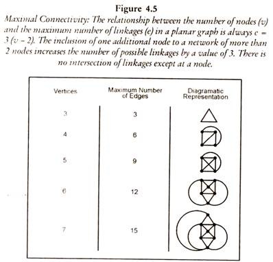
The connectivity of the network is evaluated in terms of the degree to which the network deviates from an unconnected graph and approximates a maximally connected one. The numerical range for the gamma index is between 0 and 1. This measure may be written in the form of percentage and would thus range from 0 to 100. Figure 4.5 shows the maximal connec­tivity. It is evident from the figure that for a planar graph, the addition of each vertex to the system increases the maximum number of edges by three. This proposition is true for any planar network with more than two vertices.

Cyclomatic Number:

Cyclomatic number is a different way of measuring connec­tivity. This is based upon the condition that as soon as a connected network has enough arcs or links to form a tree, then any additional arcs will result in the formation of circuits. Thus, the number of circuits in a connected network equals the total number of arcs minus the number of arcs required to form a tree, i.e., one less than the nodes or vertices. It may be written as:

Cyclomatic number = a – (n – 1)

Or

a – n + 1

Where a equals the number of arcs and n the number of nodes. This formula applies to a connected graph, where there happens to be two or more sub-graphs. Then, the formula for cyclomatic number is:

a – n + x

where x equals the number of subgraphs. This has also been expressed as:

Cyclomatic number (µ) = e – v + p

e = number of edges or arcs

v = number of vertices or nodes

p = number of non-connected sub-graphs

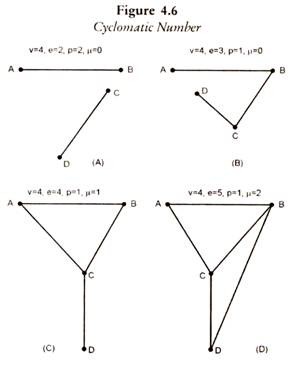
The relationship of the cyclomatic number with the network structure has been examined through Figure 4.6. Let us consider a network consisting of four nodes A, B, C, and D.

In a disconnected position or a tree type graph it has a cyclomatic number of 0, whereas as the graph move closer and closer to a completely connected state, the cyclomatic number increases. The limitation of the cyclomatic number arises since it depends upon the number of vertices and edges only.

2. Centrality within a Network:

D. Koning has developed an index known as Koning Number for describing the degree of centrality of any node on a network. The koning number for each node is calculated by adding up the number of arcs from each other node using the shortest path available. For example, in Figure 4.7, point D has the lowest number and is, therefore, the most central node in the network.

3. Spread and Diameter of Networks:

Kansky has developed two useful indices to measure the diameter and spread of a network. These are Pi (π) index and Eta (η) index.

Pi Index (π):

Kansky (1963) has developed Pi index (π) for the analysis of transport network when the focus of inquiry is to investigate the relationship between the transportation network as a whole and its diameter. The ratio between the length of the network and the length of the networks diameter would always be a real number, analogous to π. Therefore, the π index may be written as:

π= total distance of network/ distance of diameter

Or

π=c/d

where c = total mileage of a given transport network

d=diameter

The application of π index to transportation network would give a numerical value which would be greater than or equal to one. Higher numerical values will be ascribed to more complicated networks and it would reflect higher degree of development of the network.

Eta Index (n):

The eta index () is quite useful when some spatial character­istic of the network are under examination. This is also indicative of spread of a network. The eta index (n) is given by the formula:

Η = total network distance/ number of arcs

or

η= M/E

where M = total network length in kms

E = the observed number of edges

Because the numerator is measured in kilometers, therefore, the ratio is not scale free but represents the average length of an edge of the network. This index is useful in examining the utility of a given transport network. Kansky (1953) has used this index in analyzing the transport network data for a number of countries.

4. Detours:

The straight routes between two places or direct routes (also known as ‘desire line’) are the routes, which travelers used to follow because of their shortest distance. But straight routes are, however, seldom to be found in reality; even the most direct route in practice deviates from straight line. This type of deflection is very common due to physical obstacles. Such deviations can be measured by the detour index where:

Detour index= actual route distance/ straight line distance × 100/1

In other words, the detour index is the actual journey distance calculated as a percentage of the desire line distance. In fact, the actual route distance is almost always longer than the desire line distance, then the detour index will be greater, in almost all cases, than 100 and in the nature of things can never be less than 100. It is obvious that lower the detour index, the more direct is a given route. The detour index is used for assessing the effects which the addition or abstraction of links produce in a given network.

Accessibility:

One of the most important attributes of a transportation network relates to accessibility, and the geographer is particularly concerned with accessibility as a locational feature. (Robinson and Bamford, 1978: 78). When examining a transportation network, a geographer is also interested in node-linkage associations in terms of accessibility.

The structure of a network, changes in response to the addition of new linkages or the improvement of existing linkages. These changes are reflected in changes in nodal accessibility. The measurement of nodal accessibility is based on graph theory.